Mathematical Analisys
- Modelador

- 7 de out. de 2019
- 3 min de leitura
In our preview post, we studied two growth patterns betwen species and how it depends on the species behavior and lifestyle. In this document we are going to take a look on the mathematical modeling behind this growth pattern of one species and the theory behind predation.
Simulation of one species population
Single Specie Population:
As seen in the previous post, we can have a projection of the behavior of one single species growth patter, as you can see on the following image:

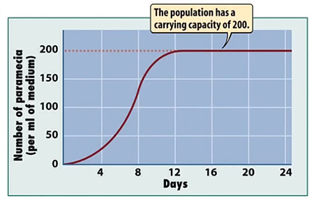
This model is based on a single species system and its carrying capacity depends only on the amount resources available for this community. This model follows a logistic growth and can be mathematically expressed as :
DN/DT = Rmax * N * (K - N)/K
Where K is the carrying capacity of the system, N is the number of individuals in a determinated time and R is per capita growth rate.
The solution for this equation is :
N(T) = K/ (1 + A*e^(-bT)) ; where A = (K - No)/No
Using the software Octave and applyting the following conditions we were able to plot a graph that describes a population growth:
K = Carrying Capacity = 1000
No = Initial Population = 100
b = Growth rate tax of this species = 1
The code created to plot this graph is:
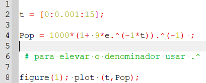
And the graph is :

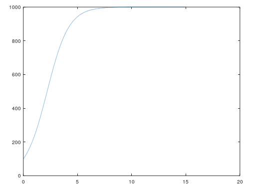
We can see that the initial population was 100 individuals and as they grow their growth rate decreases (DN/DT) as its population gets closer to the carrying capacity(1000). When the population reaches the carrying capacity the system keeps stable and invariable.
Modeling Predation
History:
This growth pattern model was first developed by Umberto D'Ancona and Vito Volterra in the year of 1920. They observed that the amount of some fish species on the fish market was highly related to its sell price. The more fish of one arbitrary species was on the market, the lower was its price. They took this observation on the fish markets of Fiume, Veneza and Trieste. During the war (1910-1923) the fishing activity was prohibid on the Adriatic Sea, leading to a higher frequency of somes species on the fish market and a lower frequency of other species on the fish market.


The data showed that the frequency of some predators, as the shark and manta ray, had increased. Observing this ,they could see that the relative frequency of their preys had decreased in the period. After they gathered all the data, Vito Volterra developed these equations to describe the dinamic of this system.
Mathematical Modeling
We need to have in our minds that this model works only for a predation relation. Other types of interaction betwen species such as competition, mutualism, neutralism, commensalism and amensalism have other formulas.
First we are going to define our variables.
N(T) = number or density of the preys in a determined time.
P(T) = number or density of the predators in a determined time.
When there is no predators, the prey population tends to grow, making its first derivative positive and will be:
DN/DT = rN ; r > 0.
When there are no preys, the population of predators will decrease, making its first derivative negative, as you can see:
DP/DT = -mP ; m > 0.
The predation tax depends on the probability of the predators to find a prey. And the predators growth rate is proportional to the probability of its predator find a prey.
So, the complete Mathematical model of this system is:
DN/DT = rN - cNP
DP/DT = bNP - mP
The frequency of the encounter of the predator-prey is given by the term NP ( Law of Mass Action).
The term cNP is related to the reduction of the prey population due to the predatism.
The term cP is equivalent to a mortality tax due to predation.
The term bNP is related to the growth rate of the predators due to the predation.
The balance points is where the variation tax of each population is zero, leading the system to an invariable state. Applying these concept to the equations we have :
DN/DT = rN - cNP = 0
DP/DT = bNP - mP = 0
Solving the equation we have two poins of equilibrium :
(N,P) = (0,0) (trivial solution)
(N,P) = (m/b , r/c)
It`s important to notice that the equilibrium of the preys depends on the predator factors (m/b) and the predator equilibrium depends on the prey factors (r/c).
On the next post we are going to approach the problem mathematically and plot the graphics of each growth pattern for predator and prey.


Comentários